Antarctic Coastal Circulations, Temperatures, and Trends

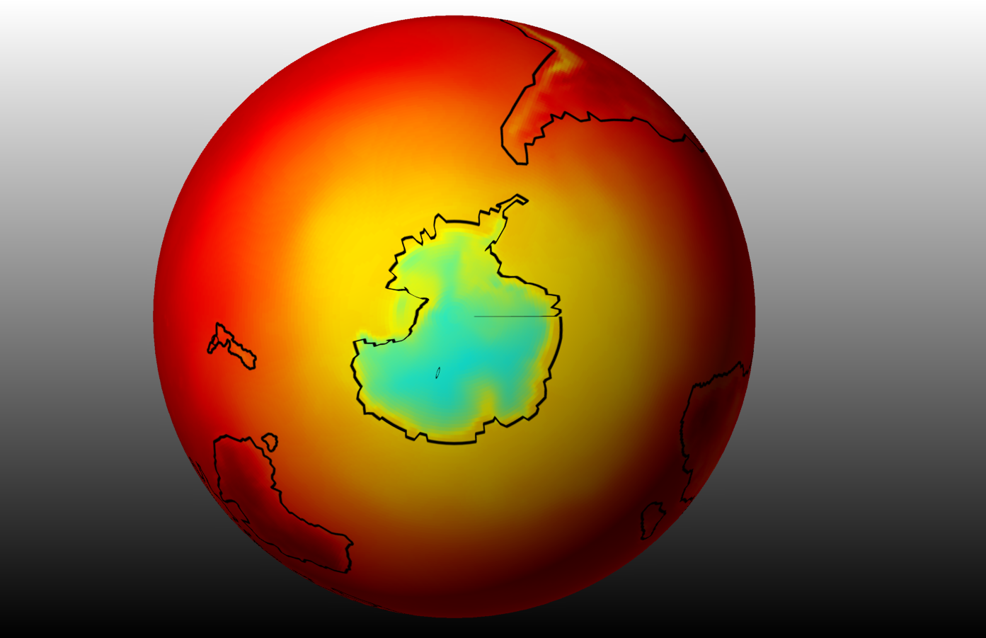
I noted in a recent post that the surface air temperature trend aligns clearly with the ocean bathymetry and all of the associated currents. The figure below compares this ECMWF-based temperature trend (left panel) to a NASA ocean bathymetry map (center panel) to an ocean current map (US Navy 1943). In the Navy map, the Antarctica latitudes were omitted, so I’ve “eyeballed” my spherical mapping. Because this is only a blog I can afford to be informal where practical and candid. In that context, I have also taken liberties with spherical mapping because I added a light source which creates darker and lighter shades that impact every color map. Readers can be expected to filter that effect when viewing all color spheres.

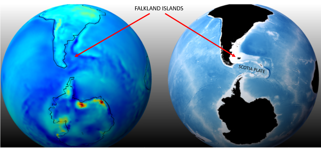
I value this historical Navy map and explore it often. The green streamlines across that (basically*) geostrophic map, represent cold currents and the orange streamlines represent warm currents. I’ve oriented the views to emphasize the interesting Falklands Plateau and Drake Passage regions that lie between South America and Antarctica.

left: 40 year surface temperature trend. Darker blue shades designate regions that have cooled the most over the past 40 years. center NASA bathymetry. right Navy ocean current

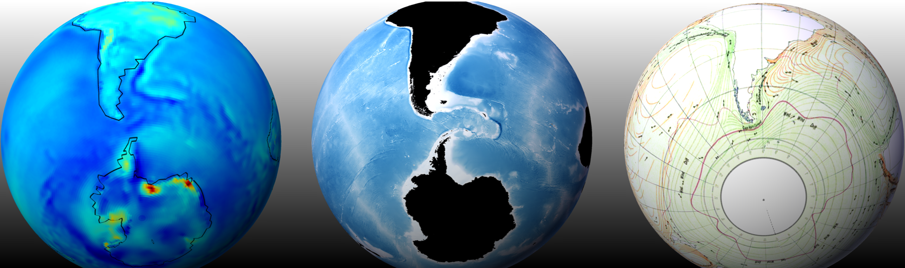
Many might agree that along with all of the subsurface topography, ocean boundaries with islands and coasts are more evident by the temperature-Trend signal, than by any ocean-current map at this scale.

Overall, the global surface air temperature trend map indicates a strong correlation to ocean bathymetry and also to ocean upwelling and downwelling. Those may explain those cool wrinkles in the left image. The key to interpretation may lie in this intriguing paper [1], especially Figure 1.

Many researchers and authors have also commented on the Scotia Plate which looks like a smear of the subsurface, pushing sediment to the east. I guess it is known to signify among other things that the underlying magma circulation follows the same Coriolis patterns that both the atmosphere and the oceans follow. In other words, the magma appears to flow in the same direction as the Southern Ocean at that latitude.

And what of the fractured crust that separates this circulating magma from the circulating ocean through Drakes Passage? Again this Drakes Passage study is very interesting and rich. A blog can jump to a preliminary conclusion that the Shackleton fractures continue to heal, and so the amount of magma – fed heat exchange to the ocean has reduced. That might be signified by the deepest of the blue shades in the left images. Or maybe just nonstationary circulations and cool creases.

These interesting signatures of the bottom of the ocean, expressed uniquely through a trend of the surface temperature variable can be compared to the vertical and largely orographic jets of coastal air seen as hydrospheric manifolds. Here, the color significance is for a profile along 75N of winds only. The vertical and the horizontal nuances of winds are captured purely from data. As for the previous image, the strongest upwelling can be differentiated from the strongest downwelling, so long as one recognizes that each figure has its own scale bar and hemisphere (and more). I’ve added a vector field which adds information and produces a complementary signature.

The images at that post and the wrinkled deep-blue patterns in the temperature trend maps here might also support an orphaned but not controversial notion that upwelling of ocean waters are accompanied by a great deal of cooling and outgassing of carbon dioxide over the satellite era at least. Yet most climate scientists appear to believe profoundly that the Antarctic and the Southern Hemisphere are bell-weathers and that those poles have been significantly warming

As the past few posts here highlight, temperature is tightly connected to circulation. Air sometimes cools when deep ocean upwelling occurs. And when a warmer air mass shifts to the north, the newly – submerged surface under that footprint becomes warmer. This isn’t rocket science. But take a look at any of these images of what I again term the hydrospheric manifold. You’ll possibly agree that coupling chemistry with the circulation of air and water over global scales of time and space is perhaps more challenging than rocket science.

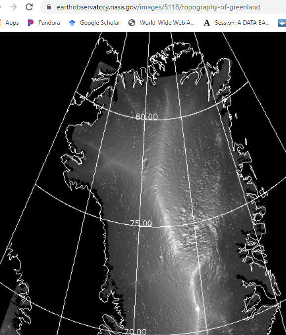
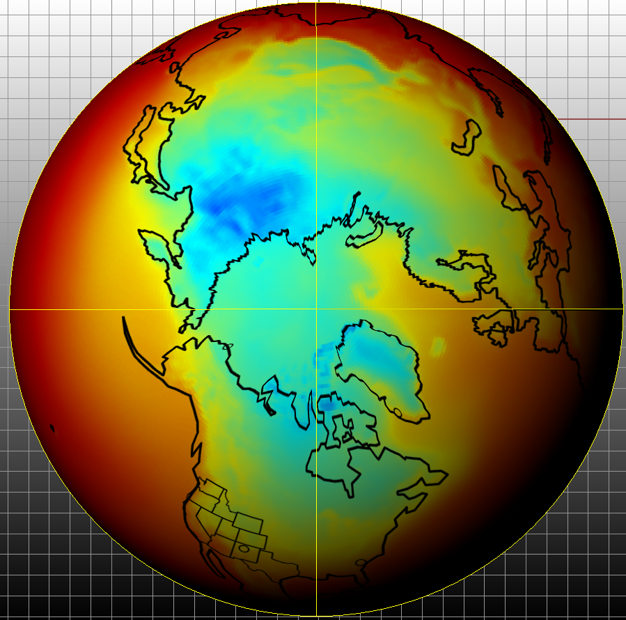
Any who follow the data and physical sciences, including where they relate to winds and temperatures, might transect at least some of this terrain. That includes these interesting vertical wind patterns. Here are sampled hemispherical plots of vertical velocity for January 1979 from the same ECMWF resource. As for the previous profile, the red hues signify high positive vertical velocities and the dark blue hues signify the opposite. The 75N latitude line crosses through Greenland.

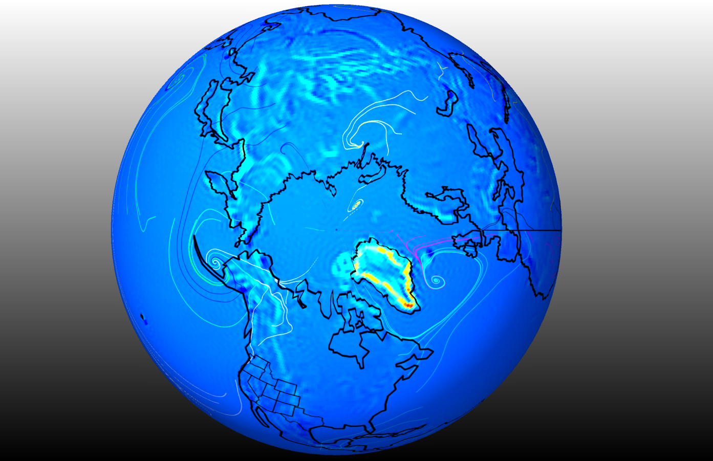
The streamlines emerge from different longitudinal lines. Spirals then signify convergent flow. Now I feel obligated to explore the geostrophic streamlines for these same vertical wind contours as shown in the next slide

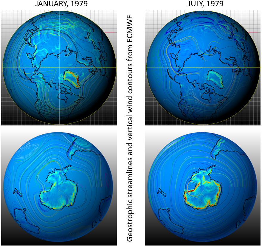
In these images, the lighter or redder the color, the greater the upward wind velocity. That typically signifies buoyant uplift of heated air. The ring of elevating air around Greenland and Antarctica is somewhat demystified for me at least when I visit this remarkable NASA page. The color fields above show a both unsurprising, yet remarkable orographic fidelity to this stone in the current.

When it comes to wind and water and temperatures, one can almost never look at too much, and so here is a two frame animation of the geostrophic (purely horizontal integration) winds with red as highest magnitude and deep dark blue as lowest, for both poles for 1979 and 1985. The circulation patterns do not fail to interest.

The vortexes at each pole, seen via the streamlines, expand and contract in synchrony over time, apparently. I’ll hold off on my July example, it’s just too graphically distracting. Again, winds both vertical and horizontal are found to transport heat, and accordingly to influence temperature and its global trends. For example, the expanded horizontal wind streamlines (the vortex) shown above for the same month seem to explain why Siberia was so cool over January 1979.

Surface temperatures across the Arctic and surrounding latitudes can have great contrast at times and so it would also be good to plot Surface Temperatures vs Geostrophic Winds. This next two frame animation is not that, but in any case, here’s a related example of geostrophic temperatures and winds from an earlier post:

It’s a very illustrative animation because for example, I noted that the Arctic ice pack shrinks and expands as the vortex does. Guess what? Polar and Ocean scientists all know this. Why can’t they share? I certainly agree that the data show the northern hemisphere is warming. I wanted to get on the same page with many in this field, because the actual cooling Antarctic data might contradict the warming claim over the Antarctic.

Or it might not. Perhaps studies somewhere describe that much of the cooling seen across the Southern Ocean, if not all of the Antarctic and its suburbs can be attributed to a naturally ongoing reduction in magmatic conductive heat flow through the aging crust, and into the cool ocean bottom. A cooling set of fractures would show up in a trend map like this.

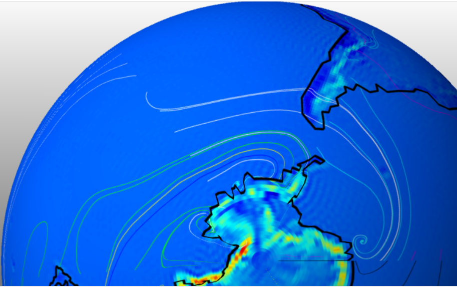
Finally to close these wind and temperature thoughts, here is the surface temperature field (not the trend field) for the Antarctica summer of January 1979. The vertical winds align with the coastal warm regions and the colder interior expresses the same outline as the outline of the dark blue fields in the wind map. The same connections apply for the Antarctica winter in July. In other words, Antarctica has relatively stable temperatures and winds.

This post explores multidimensional planetary scaled streams of air, water, magma, and many climatic signatures thereof. Any are invited to compare this perfectly transparent study to popular works which claim that our planet’s climate is one tipping-point away from cataclysmic developments. With tipping points, the conclusions can remain perfectly frightful, even as the observations remain perfectly normal.

BONUS closeup of vertical winds and geostrophic streamlines from surface

*Many must pay this price of giving up about a third of our upper atmosphere in order to work with longer satellite reanalysis times series than the previous revision of this ECMWF product. I don’t know at this point why atmospheric coverage is now so limited.

REFERENCES

[1] Krapivin, V.F. and Varotsos, C.A. 2016 Modelling the CO2 atmosphere-ocean flux in the upwelling zones using radiative transfer tools. Journal of Atmospheric and Solar-Terrestrial Physics. 150 47-54

10826total visits,2visits today